Support page
-

Can’t find it here. Click image to Contact TJS
——————————————————-
- TJS Trading Plan assistance
- TJS Goals & Progress article
- TJS Getting Started page.
——————————————————-
TJS Updates (click for update and Changelog info)
TJS Upgrade (need the “All-markets” version?)
Support Categories
Product sheets
Accounts sheets ⇓
Accounts sheet
New to TJS?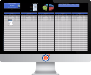
If so, please view the instructional pop-up message at the top-left of the Accounts sheet.
If you have Multiple Accounts for a Specific Market, or trade Multiple Markets per Account, please view the “Alternatives” section at the bottom of this category.
Prior TJS user?
If so, the “v8” Accounts sheet has been revamped. Please view the instructional pop-up at the top-left of the Accounts sheet.
Changes:
- The Accounts sheet no longer has a “Link-to” button, so it will not directly link to any other sheet (although it’s still possible). *
Where do I enter my beginning Account Capital?
- Go to the following cells in your Trading Log(s):
- Stocks, Options, Futures, SpreadBetting, CFD (cell AU14)
- Forex (cell AW14)
- After entering your Account Capital, you’ll also see it listed at the top of your corresponding Analysis sheet, allowing you to more accurately get the following stats:
- Current Value
- Value Difference
- ROI (Return on Investment) %
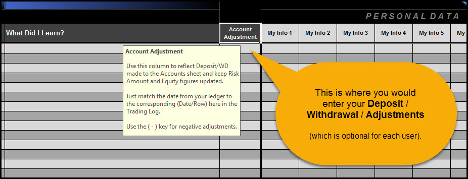
- With this method, you’ll list any Deposits (and/or) Withdrawals in the same column, labeled “Account Adjustment”.
TIP – Click in both (red triangle) pop-up messages; one in the Account Adjustment cell, and one directly above it.
* Alternatives
What would you like your Accounts sheet to do?
1) I want to sum the total of my multiple broker/accounts to my Analysis sheet(s).
We can do this by using a simple formula in one (or all) of your Analysis sheets. To do this, go to your Analysis sheet, and then click in the Account Capital cell at the top of the sheet. Now, click in the Formula Bar at the top of the Excel app. You’ll be entering a formula that will sum total the combined Capital you have for two (or more) accounts.
Here’s the formula to Sum Total all (5) accounts in to one Analysis sheet:
- =Brokers!J2+Brokers!J3+Brokers!J4+Brokers!J5+Brokers!J6
Whereas “ J2 ” equals the 1st broker, “ J3 “equals the 2nd broker, and so on.
So, if you only wish to Sum total the first two accounts, then the formula would be: =Brokers!J2+Brokers!J3
Once your formula is entered, click Enter on your keyboard – you’re done.
Sum the Total of Multiple Accounts >>
2) I trade “Multiple Markets” under the same broker/account, so I’d like to link my one broker/account to multiple Analysis sheets.
Go to your Accounts sheet. In the blue “Account 1” cell, re-enter your actual Account/Broker name. Then, underneath that enter your start date and then your beginning account capital (usually, this is the amount in your account when you start your TJS trade-tracking).
Now, go to each of your Analysis sheets, and then enter a formula in the Account Capital cell.
Here’s the formula:
- =Brokers!J2 (Whereas “ J2 ” equals the 1st broker, “ J3 ” equals the 2nd broker, and so on).
Once the formula is entered in each of your Analysis sheets, they will all be updated and synced together based on the information you enter in the ledger section of that particular broker account, in the Accounts sheet.
Link One Account to Multiple Analysis sheets >>
Analysis sheet ⇓
Analysis sheet (explanation / instructional)
Here are various example (images / videos) of the TJS Analysis sheet. Happy viewing…
Videos
Images
⇓ Getting Started with your TJS Analysis sheet
![]()
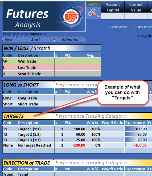
⇓ Tracking “Targets” in your Analysis sheet
– this is not a recommendation, rather an example of what can be ‘tracked’.
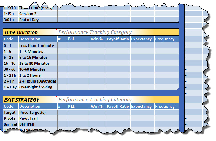
⇓ Tracking “Time Duration” in your Analysis sheet
-this is not a recommendation, rather an example of what can be ‘tracked’.
Not what you’re looking for? Request additional Images / Videos!
Trading Log ⇓
Entering "Beginning Account Balance" - VIDEO
Where do I enter my beginning Account Capital?
- Please go to the following cells in your Trading Log(s):

Elite “v8” Beginning Account Balance - Stocks, Options, Futures, SpreadBetting, CFD (cell AU14)
- Forex (cell AW14)
- After entering your Account Capital, you’ll also see it listed at the top of your corresponding Analysis sheet, allowing you to more accurately get the following stats:
- Current Value
- Value Difference
- ROI (Return on Investment) %
- With this method, you’ll list any Deposits (and/or) Withdrawals in the same column, labeled “Account Adjustment”. *
* TIP – Click in both (red triangle) pop-up messages; one in the Account Adjustment cell, and one directly above it.
Entering your 1st trade
Entering trades in the TJS Trading Log is simple, as we have added a concise column header in (row 15) of the Trading Log. If the row 15 column header still leaves you with questions, please click in any cell in row 18, were you’ll find pop-up messages that explain the trade input even further.
- Note, using the Tab key on your keyboard will make for easy navigation in moving your cursor from left-to-right in your Trading Log.
If you’d like a visual view of how to enter trades in your Trading Log, please click to view a short video.
Entering Account Adjustments
The Trading Log has a column to enter costs that are directly associated with each trade, like: (Fees, Commissions, etc). However, if you’d like to keep track of “other” adjustments, such as: (Data feeds, Platform costs, ECN fees, or monthly Dep/WD’s) without it affecting your stats in the Analysis sheet, you can do so.
Go to (and click) cell CT15 for a quick instructional message.
Here’s an example (click to enlarge)
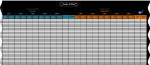
Scale (In / Out) section
We’ve chosen to keep the Trading Log as simple as possible to avoid confusion for the majority of users, so the Scale In / Out section was created, which will keep a record of your various transactions, and average out your Entry (and/or) Exit prices so you can easily paste that information in to your Price cells.
Doing this makes it possible to keep all trades on one row of the Trading Log, which is necessary for providing the best analysis possible for Strategies that involve multiple transactions per trade.
Please view this video clip for an example
Reporting sheet ⇓
Reporting sheet - Info
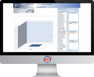 Please know, if Pivot Tables are intimidating to you, please don’t use them, or feel you need to use them to analyze your trade data. They were only included for pivot table enthusiasts, and not intended for the typical TJS user.
The TJS Analysis sheet will give you far more analytical stats then the Reporting sheets; they allow you to:
- assess your current progress,
- narrow down your Strengths & Weaknesses,
- and provide you with accurate expectancy figures,
…which the Reporting sheets will not do!
A Pivot Table report allows you to summarize vast amounts of data by categories and subcategories, as well as filter, sort, group, and explore useful subsets of data.
Each TJS Pivot Table Reporting sheet gives you a basic example of how to set up the sheet, but feel free to check (or uncheck) the boxes and experiment to see what possibilities you can come up with. There really is no wrong way to filter your data, but with that said – there are many ways to filter your data.
Tips when using the TJS Reporting sheet :
1. You can change the pivot table summary formulas by right-clicking on the pivot table (not the graph), then selecting “summarize data by” option.
2. To refresh the original data, just right-click on the pivot table (not the graph) and select “Refresh Data”.
3. To drill down on a particular summary value, double click on it. A new sheet will be created with data corresponding to that pivot report value.
4. To make a new chart from a pivot table, simply click on the pivot chart icon from the Options toolbar ribbon, then follow the wizard instructions.
Entire books have been written on the use of Pivot Tables, and the TJS staff does not have expertise in the use of the Reporting sheets. So, if you require support for these sheets (above and beyond what we’ve listed here), you will probably get a blank stare from the developer ?
Here are some helpful links if you’d like to know more:
- Click to view the Microsoft Pivot Table course.
- Microsoft overview of Pivot Tables and Pivot Charts.
Click for: TJS Reporting sheet TIPS >>
Settings
2nd Computer, Backup & Syncing ⇓
2nd Computer
If you’re looking to use your TJS on your 2nd computer, it must have the same Excel User Name (on the Excel app) that you originally installed your TJS on. *
So, please treat your Excel User Name just like any other password, or you’ll receive a registration error when using it on your 2nd (or new) computer.
- Need help with your Excel User Name? Please go to the next section (below) ⇓
* Please note, IF your multiple computers are both a (Windows and a Mac), we cannot guarantee that you will be able to share your file between the two different platforms, as there are too many variables that exist that may prevent this from happening.
Excel User Name
Excel User Name settings.
Go to the computer that you originally downloaded your TJS on. Open Excel.
Then:
- Click the File tab (upper-left of toolbar).
- In the lower left-side column, click “Options”.
- In the General tab, locate the “User Name” box. Make sure the name listed is entered exactly the same on your other computer(s).
- Once you have modified the “User Name“, you’ll need to Exit Excel and then Reopen Excel before the change can take place.
Backup to the Cloud / Syncing
![]() Older backup methods were to store files on a 2nd drive, such as an internal or external hard-drive, or a portable USB drive. However, cloud-based storage apps are now the norm and can make it ideal when using your TJS on a 2nd computer.
Older backup methods were to store files on a 2nd drive, such as an internal or external hard-drive, or a portable USB drive. However, cloud-based storage apps are now the norm and can make it ideal when using your TJS on a 2nd computer.
The most popular cloud-based storage solution, and the one we personally use, is www.Dropbox.com (receive 500mb of bonus space by using that link). Microsoft offers their own version of cloud-based storage, called OneDrive, and there are others.
- Cloud-based storage allows you to backup your TJS (and other important files), and sync those files to your multiple computers.
- With cloud-based storage (and a copy of Excel on your multiple computers), you’ll be able to easily access your TJS on each computer.
Miscellaneous settings ⇓
Macro (enable) your TJS
Macros are sets of instruction that work behind the scenes, and are used by TJS to give you a better user experience. It will be necessary to allow them to run when using the product, however – Excel gives you choices on how to enable them.
You can choose to enable macros by clicking the Excel “warning” message near the top of your sheet, or better yet… have Excel automatically enable macros (recommended)*. To do this, please spend a moment by following these instructions:
Excel (Windows) 2007 / 2010 / 2013 / 2016 / 365
- Click the File (or MS Office) button at the (top-left) of Excel.
- Click “Options” button (bottom-left).
- Click “Trust Center” (left-side).
- In same window, click “Trust Center Settings (right-side).
- Click “Macro Settings” button (left).
- Choose to “Enable all Macros…”
- Click “OK”…
- Save and Close the Excel program.
- Reopen Excel.
Excel (Mac) 2011
- On the Excel menu, click Preferences.
- Under Sharing and Privacy, click Security.
- Select the “Warn before opening a file that contains Macros” check box.
*While performing the above instructions, Excel may say this is not recommended. This is true if you commonly download Excel files from the internet and not knowing where they originate from. if so, just use Excel’s ‘warning’ message to enable macros each time you open the file.
Click for Macro Settings instructions >>
Macro Security Risk (Excel warning message)
A recent Microsoft update has disabled macros (by default) from all files downloaded from the internet.
While this can be good if those files are downloaded from an erroneous source/website, it makes it necessary for the user to enable macros when the file is downloaded from the internet. Please know, macros are needed to provide the type of features and functionality that are found in the TJS product file, which has been a trusted source since its 2009 inception.
Thus, if you are getting the following message near the top of your Excel application, please follow the instructions that follow.
![]()
- Close the TJS file/workbook.
- Right-click on the file/workbook.
- Select Properties
- Under the General tab, make sure to check the Unblock box (near the bottom/right corner).
- Click the Apply button.
- Now, open the file/workbook.
- The error message should no longer appear.
Here’s a quick video to clarify the instructions, if necessary.
[/expand]
Sheet Tabs (where are they)?
They’re hidden by design.
Older versions had both sheet Tabs and the TJS Home Menu, but we found having them both together made it confusing for many users.
The TJS Home Menu is definitely recommended for the “All-market” version, as the number of sheet tabs are too numerous, which means only a fraction of them are in view. Remember, the TJS Home Menu was created for easy navigation, whereas all sheets are neatly categorized in sections along with an image to tell you what resides in each (sheet/tab) link. *
If for some unusual reason you absolutely, positively, must have sheet tabs, please follow these instructions to make them magically reappear:
Excel for Windows
1. Click the Green File button (or the colored Microsoft button in Excel 2007)
2. Click “Options” (or “Excel Options” in Excel 2007)
3. Click “Advanced” from the left sidebar
4. Scroll down about half-way until you see “Display options for this workbook”
5. Put a ‘check’ in the “Show sheet tabs” box
Excel for Mac
1. Go to “Excel” (from the menu bar)
2. click “Preferences’
3. Click “View”
4. In the “Windows options” section, put a check in the “Show sheet tabs” box
Click for: Sheet Tab instructions >>
* Some Microsoft Mac users have had issues with images displaying in their file. If you fall in this category, we have created a “text” link Home Menu version (void of images). Contact us if you need this version.
Helpful TIPS!
Screenshots & Trade Review ⇓
Link screenshot images to your trades
 First, you’ll need a screen-capture utility like Snagit, or Windows “Snipping” tool.
The TJS has a handy TJS Chart/Image maker as well (linked from your Trading Log header). It’s more time-consuming then Snagit or the Snipping tool, but it has lots of annotation and editing options.
Once you create your link, it’s recommended to save it in the same folder your TJS resides in. Also, make sure you don’t (rename or change) your image name or folder location. If you do, you’ll invalidate your links. *
After saving your screenshot image, link it to any cell of your spreadsheet* (the cell must have text in it).
* We suggest you link it to the Symbol column in your Trading Log. By doing so, the TJS Trade Review sheet will attempt to display your image in the image box location.
⇒ “Hyperlink” instructions:
Once you create your link, you’ll need to make sure you don’t (rename or change) your image name or folder location. If you do, you’ll invalidate your links. *
1. In the Trading Log, Right-click the text in the Symbol column, and then choose Hyperlink on the shortcut menu. An “Insert Hyperlink” box will pop-up.
2. Locate your saved (image) file.
3. Click on the file name of your image — Click OK.
4. The text you hyperlinked is now (blue/underlined). Clicking it will instantly open up your picture viewer and the image you associated the link with.
5. Your done! *
Now, go to the Trade Review sheet to review your trades and compare the charts with the notes you recorded in the Entry Notes / Exit Notes journal section. Comparing your notes to the actual charts that you traded will allow you to more easily determine what you did right or wrong, and what you may do differently in the future.
* Note:
If you plan to enter screenshots, decide on a file location for your TJS and screenshot Images before you start. Always keeping your (images and TJS file) in the same folder is advised, and if so… you should never experience an issue with the Hyperlink function not finding your image.
This is due to Excel needing to see a relative path to those images, which will be lost if the (image or TJS file) is moved from its original location. Although there are variables with some systems that may not experience these issues, it’s best to play it safe.
Click for Hyperlink Instructions >>
[ A short explainer video is in the next section (below) ] ⇓
Trade Review sheet - VIDEO
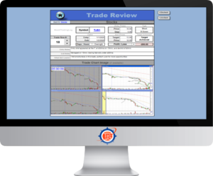 The Trade Review sheet can automatically detect your hyperlinked (screenshot) images, but in order to do so, it needs a specific column to look for those hyperlinks, which is always the Symbol column of your Trading Log(s).
Once you’ve created your hyperlink *, the Trade Review sheet will attempt to detect the linked image, and then display it in the lower section of the sheet. This will make it easy to review your trades by simultaneously referencing: your screenshot image, trade specifics, and the notes that you took of your trade.
There are two ways to access the Trade Review sheet:
![]() 1) Double-click the “Click” text, which is directly to the right of the Journal/Notes section. This will take you to the same corresponding trade row that you clicked from.
1) Double-click the “Click” text, which is directly to the right of the Journal/Notes section. This will take you to the same corresponding trade row that you clicked from.
2) Click the Trade Review button in the top-header of your Trading Log. Once there, you’ll need to use the Toggle (row #) button to locate a specific trade.
If your image is not populating, please try toggling the Up/Down arrows on the left-side of the sheet. The number listed on the left-side of the arrows is the corresponding trade-row # from the Trading Log.
* Not sure how to use Excel’s Hyperlink function? It’s as easy as right-clicking in your Symbol column, choosing ‘Hyperlink’, and then pointing to your saved image. For more information, view the faq category (directly above).
Quick Summary Info ⇓
Excel's "Quick Summary" status bar
For those that don’t know… Excel displays a very helpful summary in the (lower status bar) window. It’s a great way to get a quick P&L total for things like: Day / Week / Month.
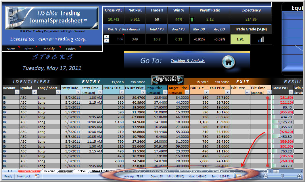
Just scroll & highlight any numeric data column and you’ll see some interesting calculations come to life, at the bottom of your Excel app:
* Sum
* Average
* Minimum
* Maximum
* Count (# of items)
- Depending on which column you’re highlighting, you may need to first unprotect the sheet [ Review > Unprotect sheet ].
You cannot permanently keep these results in your TJS, but when you want a quick answer to a question on your input area, it can’t be beat for its quick and instant display.
To change your choice of what the status bar displays (or if you do not see the Quick Summary info), just right-click on Excel’s footer bar and you will see your choices. Check or uncheck the ones you want displayed.
Click for instructions >>
Backtest method ⇓
Using TJS to Backtest strategies
 First, you’ll need to…
1) Create a duplicate copy of your product file by simply performing a “Save-As”.
- Name the copy “Backtest“, then keep the ‘original’ for live trading.
- Print the following sheets to have handy while performing your back test:
2) Trading Plan
For all steps listed (below), your back-test can only be deemed reliable if it is done (according to your plan). Your Trading Plan should be specific and tell you when to Enter the trade and at what points you will Exit your trade, either by:
- Exit the trade for a loss, or
- Exit based on a predetermined profit-taking method.
3) Trade Sheet – (found inside each product file).
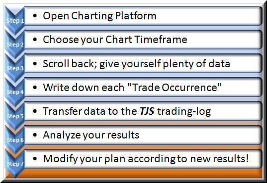
- Use this to write down your notes of each Trade Occurrence. You will transfer these notes directly to the Trading Log when you are finished.
- Alternatively, you can enter your backtest trade entries directly in the Trading Log.
- When you see “Trade Occurrence” (step 4, in image below)… you’ll be writing the “codes” in the Trade Sheet for each individual “Performance-tracking” category you wish to track, while using the Tracking sheet for code references.
4) 7-step Backtesting procedure:
Broker Importing info ⇓
TJS Importer
The TJS product is unique in that it summarizes your trade information in to multiple Performance-tracking categories, which means that getting the type of analysis that the TJS offers, manually entering your trade data may be necessary.
- However, Ninja Trader allows users to export their trading data in a nicely organized file that can be imported to the TJS Trading Log. If you use Ninja and would like more information, please click here.
- Please know that (98.4%) of TJS users do not use the TJS Importer. They are manually entering their trade data and using that time to reflect on their trading day, as mentioned in this user testimonial…
“… I tried subscribing to some online trade-tracking sites but there is nothing like taking the time to manually record your trades to really understand your game.” ~ Simon Smith, Canada
For the DIY (Do-It-Yourself) traders who’d like to try Copy/Pasting their trade information from another Excel file:
To make sure you don’t invalidate the formatting of the TJS, use the following function when pasting your information:
- Paste Special > Values (only). This will ensure that you don’t compromise the TJS formatting.
Trade Input (help)
Crypto ⇓
Crypto (Help page)
Need help with your Crypto trade entry? If so, please visit the TJS Crypto Help page.
- You can also visit this page anytime by clicking in cell E1 at the top of your Crypto Trading Log.
Futures ⇓
Contract Sizes
The Futures Tracking sheet allows you to Track & Analyze specific instruments, however, most will have varying contract sizes. Since the TJS will attempt to calculate your P&L for you, the sheet needs to know the size of each instrument that you list.
For a list of common Futures and Commodities (contract sizes), please visit the TJS Futures Contract Size page.
For Bonds and unique Tick prices
Some Futures instruments have unique pricing structures, and since Excel must have a standard numerical format to calculate, it’s necessary to enter Prices in their Decimal equivalent. If not, you’ll see (#VALUE) in the Gross P&L column.
- Download the “Converting unique Tick prices” PDF page, or continue reading on how to manually convert your prices.

For prices listed with an apostrophe in it:
You’ll need to replace the ( ‘ ) with a ( . ), and to its decimal equivalent. Example for a ZB price of 126’29.0:
- 126‘29.0, would be changed to 126.29
- then, calculate the decimal equivalent by dividing the decimal numbers by 32,
- so, 126.29 would be entered as 126.90625 (29 ÷ 32 = .90625)
For prices listed in fractional quotes (like, ZB):
You’ll need to convert the fraction in to decimal format by simply using your calculator and dividing the top fraction by the bottom fraction to give you the decimal equivalent.
- Example: 11/32 = .34375
Forex ⇓
Gross P&L
Forex involves trading a myriad of different currencies, and some of the Pairs you trade will not be quoted in your native (broker) currency.
The “v8” Forex product allows you to choose your native currency (cell G11), which means the P&L calculation will be correct for all Pairs that are quoted in that same currency; the “quoted” currency always being the 2nd currency listed in the Currency Pair.
It is important to know, the TJS does not have the ability to convert the price of non-native currencies, so…
- You will need to adjust your Profit / Loss (for currency pair trades that are not in your native currency). You can do this very easily by (manually) entering your adjusted profit/loss in the Gross P&L column. This will override the formula and allow you to enter the correct adjusted profit / loss.
Account Size
Some brokers allow you to trade an exact quantity and others have a base ‘lot’ size that is used to trade with. Basically, there may be many variances between the myriad of brokers out there, so we tried to make it as simple as possible for users to input their data regardless of what type of account they have.
- Click in cell F10 of the Trading Log. You’ll see a drop-down arrow that will allow you to choose a specific Lot-size. Please choose accordingly, then enter your contract (QTY) in column H. Once done, these two figures will become part of the Gross P&L equation (but only for USD quoted trades, as explained above).
- If you’d rather not set a specific Lot size, then choose “1” in the drop-down arrow of cell F10, then enter your contract (QTY) accordingly — in column H.
Risk Amount (column AJ)
Why are some “Risk Amount” calculations incorrect (or color coded)?
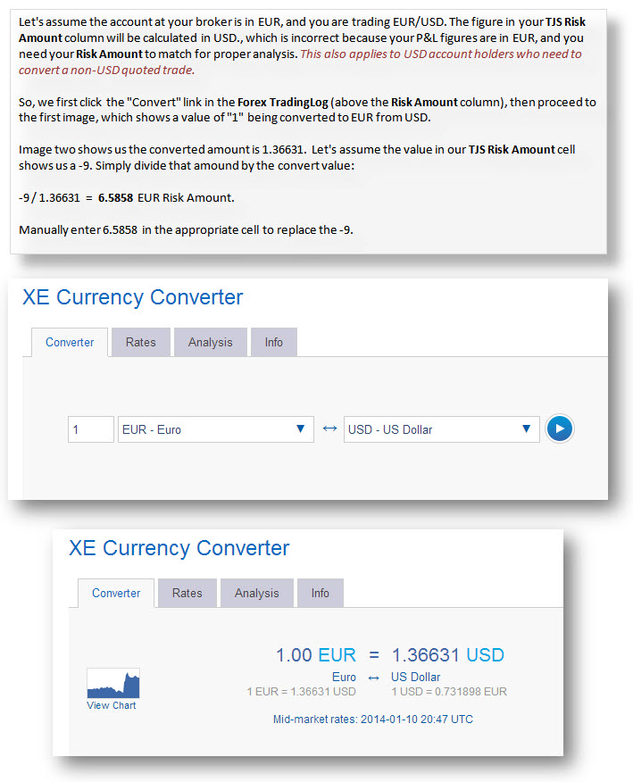
As in the case for the Gross P&L needing intervention, so will the Risk Amount if your trade is not in your native currency (cell G11).
The color-coded Risk Amount cell is a warning that a non-native currency pair was entered, and that you should verify that the figure is accurate.
If the trade is in your Native currency.
- The Risk Amount cell will automatically display your results for all trades quoted in your native currency (cell G11).
If the trade is not in your Native currency.
The Risk Amount cell will be maroon in color, and will have an amount shown that will need one of the following actions:
- “Manually” enter your own adjusted Risk Amount, or
- Click the link in cell AJ13 (directly above the Risk Amount column) for help with converting the amount shown to your native currency – click image for example.
Trade input, with Multiple Currencies
Since traders can be found all around the world, there are no default currency symbols used in the TJS.* This way, any currency will be calculated correctly, as long as all trades are in one common currency. However…
If you trade with brokers using multiple currencies, you can do one of two things:
1) Manually enter your actual P&L (in one common currency) in the Gross P&L column of the Trading Log sheet. To do this, you’ll choose your Main ‘native’ currency where all trades will be automatically calculated. Then, for all other non-native currency trades, you’ll manually enter the adjusted profit/loss in the Gross P&L column (the amount you actually made in your native currency).
You’ll also want to do this in the Risk Amount column (if using Stop-prices).
- This will over-ride the formulas and avoid having to convert prices.
2) Duplicate your product file. Then, Record each “currency type” in separate files.
- This way, there is no converting to do, and the P&L column will auto-calculate your trades without any intervention.
The Analysis sheet needs consistent P&L data, and by choosing one of these methods… all of your data will be consistent, giving you reliable tracking analysis.
* Exception – The (UK) Spread Betting TJS displays the Pound symbol in some price fields.
Options ⇓
Options Trade Input (methods)
The Analysis sheet, and its various “Performance-tracking” categories need to see “consistency” to produce meaningful data to track and analyze your results. Due to the complexities of Options trading, there are two different methods of trade input to choose from.
So, before starting with your Options trade input, you’ll need to choose a method of recording your trades. Choose the one that makes most sense to you and your trading regimen, then stick to that one method for each successive trade input.
Method 1
Each trade (regardless of the number of ‘legs’) are summed together on one row in the Trading Log.
Pros:
This is the simplest method, and recommended if you don’t wish to enter Quantity or Price information in the Trading Log sheet.
- Each (multi-leg) trade is entered on only one row, regardless of how many ‘legs’ were executed.
- Skip the (Entry – Stop – Target – Exit) columns.
- After ALL ‘legs’ of the trade are closed, sum the Profit/Loss, then manually enter your Gross P&L.
- The trade (as a whole) gets classified as one single strategy in the Tracking Codes section of the Trading Log.
Cons:
Without Entry and Exit price information, the Open and Closed Equity calculations in the top header won’t populate, and the following information in the Trading Log’s “Trade Summary” section will not populate:
- Risk Amount — R-Multiple — Reward-to-Risk — % Gain
- This is offset by getting some very detailed analysis in the Analysis sheet.
Example images of both Trading Log and Analysis sheet, for Method 1:
– Maximize the browser window for an enlarged full-screen image
Method 1>>
Method 2
Each trade ‘leg’ is entered on separate rows in the Trading Log.
Pros:
Since both Quantity and Entry & Exit price information is required, TJS will automatically sum your Gross P&L, along with additional fields in the “Trade Summary” section (if Stop and Target prices are entered).
Cons:
Since each leg of the trade is entered as its own trade, your Win % analysis in the Analysis sheet will likely reflect both winning and losing percentages for a single trade regardless of the outcome of the trade (as a whole).
Example images of both Trading Log and Analysis sheet, for Method 2.
– Maximize the browser window for an enlarged full-screen image
Method 2>>
Help Me Choose!
Which Method (#1, or #2) is best for me?
TJS set out to ease the burden (or the complexities) of Tracking & Analyzing Options trades, but that does not mean it’s a one-size-fit-all approach. Before we can start tracking our Options trades, we need to figure out one of two Methods of trade input.
Personally, I always try to keep things simple and if that’s what you’re after, consider using method #1, but keep reading to understand if the ‘simple‘ method is truly for you.
While I do find that some Options traders use #1, the majority choose #2, as it provides additional (per trade) analysis in the Trading Log sheet; however, the Analysis sheet stats will be slightly skewed when looking at the Win % and the Payoff Ratio. This is in part to having strategies with more than one leg, where one (or more) legs may be a Win while another leg was a loss. As long as you understand this nuance, the “Expectancy” column will be your best Performance Tracking Category (no matter which Method you choose).
Here are some important questions to consider before deciding to commit to either input Method:
1) Do you need TJS to show you Open and Closed Equity amounts? – Your trading platform may already tell you this.
- If so, #2 may be for you.
2) Do you enter Stop and Target Prices? – Which opens up more calculations in the AH -> AK columns.
- If so, #2 may be for you.
3) Do you trade Covered Calls?
- If so, view the next faq category (below) to read an excerpt of why C.C. traders may wish to use #2. ⇓
If none of these points are relevant, then I’d opt to keep it simple and use #1.
Click to, Help Me Choose>>
Covered Calls
It is important to note that the TJS staff does not actively trade Options. So, we have asked for help from the TJS user community (ones who are avid Options traders) and they have kindly provided the excerpts below. We hope you find them helpful, and if you would like to add your own write-up or add to an existing one, please send us a message.
Covered Calls – with fellow TJS user:
Avid Options trader, Bonnie Hayworth says…
“Some traders wish to see their total P&L combined on one Trading Log row (Method 1), which is not possible with (Method 2) and that is a good thing. I like to break it out using Method #2 to see how well selling premium is working against each product and more importantly, when selling premium makes sense! Here’s why; say you own SLV and APPL, and SLV moves sideways a lot of the time. Silver and gold run cyclically in the Market place, and they typically move higher in the latter part of summer. With that said, I am able to track on the the TJS that selling calls on SLV in the month of August and September is a bad idea… that my probabilities are very low in those months.”
Input:
I input this as two transactions (separate rows in the Options Trading Log) because that’s how it played out. This will show in the P&L (if /when) the stock is sold. It’s the opposite in the sold call depending on if the stock is already owned, which will dictate the way the transaction is inputted.
If you have the TJS Stock/Options product, then you may wish to enter your Options – Covered Call “Stock” transactions in the Stock Trading Log – this will be a personal preference.
If you have the TJS Options product (only), you’ll enter your Covered Call “Stock” transactions in the Options Trading Log. To get the proper P&L for your Stock trades, follow the instructions in cell N11 where it says “Adjust Size” — this will change the Contract Size back to Share size.
Click for more info >>
Exercise / Assignments
It may be a personal preference whether you choose to log “Options Assignments / Exercises” as a Stock trade (in the Stock Trading Log) or keep it in the Options Trading Log. Our thoughts are to always keep it simple in the name of providing the best analysis for ‘you’.
There are two main preferences…
1) Close (and/or) Open the Option position in the Options Trading Log by entering a .00001 in the Exit Price column, and then enter the new position (on a new row). Make sure of the following… in your Options Analysis sheet, you should have an Entry Strategy (Code and Description) that includes the possibility of an “Assigned” position.
The Entry Strategy for this type of trade could, for example, have a Code and Description of:
- Code: A.O.P.
- Description: Assigned Option Position.
Now, ‘tag’ the trade accordingly in the Entry Strategy column of the Trading Log (below the blue Equity-curve graph) so the trade will appear in the Options Analysis sheet once the trade is finally Closed (with a Gross P&L entry).
2) Or, treat it as a new Stock trade if you have one of the following TJS product versions: (Stock/Options or All Markets). If this is your preferred method, then you would create any new assignments in the Stock Trading Log.
The Entry Strategy for this type of trade could, for example, have a Code and Description of:
- Code: A.O.P.
- Description: Assigned Option Position.
So, do whichever makes most sense to you and your trading style, and then remain consistent with it for each and every similar trade to achieve optimal analysis.
Click to view the Preferences >>
Stop and Target prices
Please know, entering Options Stop and Target prices is optional. If you decide to enter Stop and Target prices, please continue…
Because Option prices are not linearly related to the underlying stock prices, there is no way to use the underlying Stock prices directly to produce a risk (and/or) reward amount for an option trade.
What the TJS user can do is use the “delta” value of the option to help evaluate the risk and reward scenario. For a long position, estimate the “stopped out” value of the option by multiplying the number of points, by the “delta” of the option that was chosen. Subtract this amount from the option purchase price.
The following example should help:
Suppose a stock price is at $20.00 and you have purchased a $17.50 Strike in the money option for $4.00. Suppose the “delta” for this option is .75 (The option chain should give the actual value.)
If you want to set a stop loss based on the stock price dropping to $18.50, you’ll need to calculate what the value of the option would be when the stock is at $18.50. There are option calculator tools that can do this but a quick way is to realize that for a stock with delta of .75, a $1.00 drop in stock price will cause a $.75 drop in the option price. So for a $1.50 drop in the stock price — $1.50 x .75 = $1.13. So when the stock is at $18.50, the option is worth approximately $4.00-1.13 = $2.87.
For the reward (Target) side of the equation, you can just estimate at what value you would be willing to sell the option, or if you want to tie it to a particular stock price, you can do it the same way by adding the option’s delta to its price for every $1.00 move in the underlying stock. This is complicated when the stock moves more than a couple of points, because delta will also increase along the way. The best way may be to look at what you paid for the option, then look at what your risk is and set a target price to sell the option at purchase price plus – 3(x) what your amount of risk is. So in this example you would estimate a stop loss value of option as $2.87, and estimate target price of option as $4.00 + (3 x $1.13) = $7.39, which gives a 3:1 reward / risk ratio.
The long and short of it is that, unlike stock prices, option prices do not correspond in a linear manner to the stock price. If you want to do the calculations exactly, you’ll need to evaluate the value of your particular option at your “Stocks” stop loss price and target price.
You may find it sufficient to use a quick head calculation of the effect of delta to set the value of the option at the stock stop loss point as described above and to set an arbitrary value for a target sell price of the option. This should permit a good enough risk and reward calculation in your spreadsheet for most purposes.
Click to view examples >>
Contract Size function
In your Options Trading Log, there is a section in the top-header that allows you to do the following:
- Change the default Contract Size – for (all) trade rows.
- Change an individual row’s Contract Size – for entering a Stock trade.
Instructions are included in that section. Just hover your mouse cursor over the small red triangles to view.
Binary Options
Recording and Analyzing your Binary trades should be no problem in your TJS. If you’d like to keep these trades separate from your other conventional Options trades, then just make a duplicate copy of your TJS (rename it accordingly).
![]()
- Click the thumbnail to view the “Analysis sheet for Binary traders” example.
- then (click the image to enlarge).
(UK) Spread Betting ⇓
Spread Betting (Currencies)
When trading the usual Pound per Point trades, the input is all standard and self-explanatory. However, if trading SpreadBetting currencies, please read on…
Enter the following in the Entry Qty – Column F, depending on what type of trade it is:
- SpreadBet (no currencies) ” 1 ” for each pound, per point.
- SpreadBet (JPY quoted Currencies) ” 100 ” for each pound, per pip.
- SpreadBet (all other Currencies) ” 10,000 ” for each pound, per pip.
- or, see alternative (below image) *
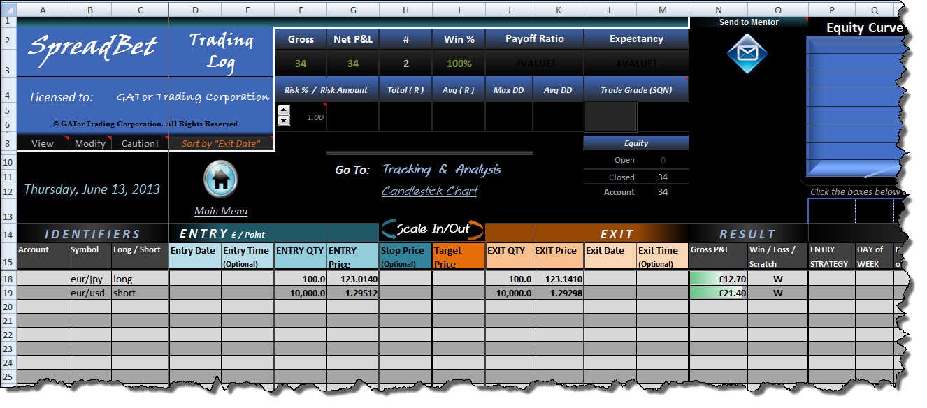
* Alternative – manually enter the correct P&L in the Gross P&L column (over-righting the formula).
Troubleshooting
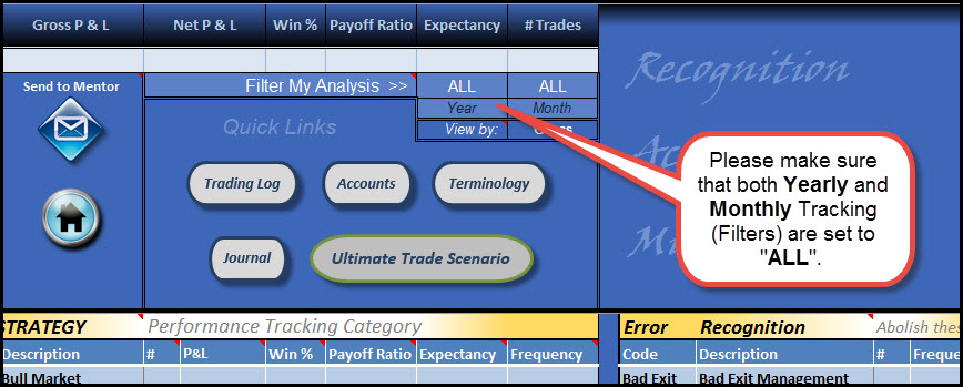
Analysis sheet is not displaying all of my trades
Are you missing data? It may be your filter. Click to view the following image…
Microsoft Support ⇓
Microsoft - Update Links & Support Info
Microsoft Update Links
Windows Update and Mac Update are the recommended ways to update, for all MS applications.
Individual Excel Updates (for older MS Excel apps):
- Update Excel 2007. (no longer supported as of May 24, 2019)
Microsoft Support Page
- Microsoft Contact Us.
Microsoft Technical Support
Windows Excel
- In the US, call (800-642-7676).
Mac Excel
- In the US, call (866) 474-4882. In Canada, call (800) 936-8479.
Excel (specific version) Troubleshoot Links:
Microsoft (Office 365) Troubleshoot Links
- Excel not responding, freezes or stops working. Microsoft Crashing and not responding help page.
- Repair a corrupted workbook for Office 2013 / 2016.
- This may be necessary if one of the internal files needed to function a specific aspect of Excel becomes damaged, deleted or corrupted during a brutal shutdown.
- Microsoft Office 365 Easy Fix
- If your Office 365 or Excel (2013, 2016) is not working correctly, try restarting it to see if the problem is fixed. If not, try repairing it with one of Microsoft’s “Easy Fix” tools.
- Repair an Office application
- When trying to repair Microsoft Excel from your computers Control Panel, use this.
- Recover a corrupted workbook
- If Microsoft Excel detects a corrupted workbook when opening, it initiates File Recovery mode and then attempts to repair the file. If File Recovery mode doesn’t start, try using this manual process to recover your file.
- Automatically Save a backup of your workbook
- With a backup copy of your TJS file, you’ll always have access to your TJS even if your workbook is deleted mistakenly, or if it becomes corrupted.
- Automatically create a recovery file at set intervals
- A recovery file also helps to ensure you have access to your data if your TJS is deleted mistakenly, or if it becomes corrupted.
- Uninstall Office 2013 / 2016 or Office 365 from a Windows computer.
- When all other solutions have been exhausted, or none exist, it’s best to fully uninstall Office/Excel 2013 from your computer, wiping it clean of all potentially corrupted files that may be left on your Windows set-up. – Click the link to have Microsoft do this for you.
- Office 365 frequently asked questions.
- Applies to Excel 2013, 2016, Office 365
Microsoft (Office 365) Troubleshoot Links >>
Microsoft (Excel 2010) Troubleshoot Links
Excel 2010
If your Excel (2010) is not working correctly, try restarting it to see if the problem is fixed. If not, try repairing it:
- Go to your Control Panel > Programs and Features, right-click on Microsoft Office 2010, and select Change.
- On the next screen select Repair. Microsoft Office will go through and do a repair and hopefully that will get you up and running again.
Microsoft (Excel 2010) Troubleshoot Links >>
Microsoft (Excel 2007) Troubleshoot Links
Excel 2007 Fix It
If your Excel (2007) is not working correctly, try restarting it to see if the problem is fixed. If not, try repairing it with Microsoft’s “Diagnostics” tool. Here’s how:
- In Excel, click the top-left Microsoft button > click Options (bottom) > click Resources (left side-bar) > click Diagnose (right side-bar).
Microsoft (Excel 2007) Troubleshoot Links >>
Microsoft (free) Security
Windows Defender
Included for free with Windows 8, 8.1, RT, Win 10.
- If you are not running an existing Anti-virus program, make sure you enable it. Type in “Windows Defender” in your Start button ‘search’ bar, then configure (if needed).
Microsoft Security >>
Mac Limitations ⇓
Mac 2011
A few of the cells don’t look formatted correctly
The TJS incorporates merged cells in some locations of the file (when necessary), but the Mac Excel software app does not display all of them properly, which…
- Gives an awkward appearance to some formatted cells (mostly in column headers). If you notice colors that don’t quite match the surrounding cells – this is the reason – but nothing to be alarmed about.
Most of these issues have been fixed in the “v8” product version.
Cells don't look formatted correctly >>
Trade Review sheet, “Comments section may not expand (or will truncate) the text.”
Unfortunately, this is not an issue we have much control over. The TJS has gone through extensive re-coding to be as “Mac” compatible as possible. This is one of those issues that Mac Excel 2011 is not able to interpret the coding as its Windows counterpart does.
Trade Review sheet > Comments don't display properly >>
Yellow headers in Analysis sheet do not automatically change the corresponding headers in the Trading Log.
This does not apply to Windows Excel users!
- Go to your Trading Log, unprotect the sheet and manually enter your new category header name in row 15, under the “Tracking Codes” section (which is under the Equity-curve).
Trading Log > Tracking Codes header section is not updated from Analysis sheet >>
Accounts sheet “Link-to” button (“v7” product users).
Not all Mac users will be able to utilize this function.
An easy workaround is to simply enter a formula in the Account Capital cell of your Analysis sheet. For example, to reference “Broker1” in the Accounts sheet, you’d go to your Analysis sheet and enter the following formula in the Account Capital cell (very top):
- =brokers!h2
To combine the total of more than one broker, just add to the formula, like so:
- =brokers!h2+brokers!h3
Accounts sheet > Link-to button doesn't work >>
Mac 2016 (and greater)
Since 2016 came out for Mac, some users have experienced issues with their Mac Excel 2016 / Office 365. None of these issues are critical and in no way hamper your ability to analyze your trades as TJS intended!
Hopefully with ongoing Microsoft for Mac updates, these issues will be fixed. For now, there are work-a-rounds.
Aesthetic limitations:
Some “Images” may not display (or may appear as a Red X, or something similar)
This is a known Mac 2016 “layering” issue. If you are affected by this, please contact TJS. We will send a new modified “Mac” file that addresses this issue.
“Pop-up” Comment messages (from the small Red triangles) remain hidden under objects
For instructional purposes, the TJS incorporates pop-up comments in key locations in each sheet, which can be hidden from view by nearby ‘objects’ (Images, Buttons, Graphs, etc.) located near the pop-up comments.
- If your Mac Excel 2016 has this issue, please contact TJS. We will reply a new modified “Mac” file that includes all affected pop-up messages.
Aesthetic limitations >>
Other non-critical functionality limitations:
Deleting market sheets (Home Menu)
If this functionality does not work, please do the following…
- Click “Abort” to close out of the error message.
- Close the file and then Reopen the file.
- Most users have reported that the function will now work.
Options Trading Log
If you receive an error message when clicking in a Gross P&L cell, or when clicking the Filter buttons under the blue graph, then…
- Click on the upper Review tab, and then Unprotect sheet. The error message should no longer appear.
Data-transfer function
Most users will never use this function.
- So far, there is no work-a-round for this function, other than to manually copy the data from the old file (to the new file) using the Copy > Paste Special > (Values only) to paste your data. This is not always recommended because of the potential to compromise the new file. The only other option is to start ‘anew’.
Other limitations >>
Errors
Error messages ⇓
Error Messages (various)
Please know, encountering an error message is extremely rare, and usually occurs when there is an issue with the host computer. Thankfully, we have been able to successfully troubleshoot most (if not all) of the issues that we’ve been notified of.
— Below are the error messages that TJS has fielded to date —
TJS crashes after entering data in the Trading Log or Analysis sheet
The cause is most likely a recent upgrade to Windows 10. Although it’s not understood why it happens with this particular O/S upgrade, we’ve identified an Excel setting change that will cure the issue:
1. In the upper toolbar, go to File > Options > Advanced
2. In the Editing Options section, clear the checkbox for “Automatically Flash Fill”. Go to the next step…
3. Click on the General tab.
4. Clear the checkbox that says “Show Quick Analysis Options on Selection”
TJS crashes after entering data in the Trading Log or Analysis sheet >>
##### signs
This is not an error or malfunction… just an Excel warning sign that the column is not wide enough to display the figures in the cell. This happens because of the difference in screen resolutions between computers.
Go to the top column header, and then double-click the right-side of the column header. It should automatically widen it to display your data.
- If your sheet does not show the upper (letter) header, Go to the upper toolbar and click on View > Headings (check the box to view the column headings).
##### signs >>
Restrictions on this Computer
(Also applies to, “Your organization’s policies are preventing us from completing this action for you.”)
First, be aware…
- If you are using the TJS file on a work computer, your working environment may have security restrictions. If so, please try it at home (where your system will not have these added restrictions).
To fix…
- Are you using an older Excel version? If so, it may need updating. Security updates happen often to keep you safe, and certain files will not open without these updates. If you are not sure if your system has the latest updates, please click for windows updates, then read on below.
- Try using the Microsoft Easy Fix support page, which handles this (and other) issues. This should cure the problem – it has for everyone else with this issue. The most likely fix to try is the, “Find and fix problems with connecting to the Internet or to websites”.
- Do you have a default browser set? Sometimes browser apps are uninstalled, leaving no browser default that the link can associate with. If this is the case, simply go to your existing browser settings, and set it as your default browser.
Restrictions on this computer >>
The File is Corrupt and Cannot be Opened
This happens very infrequently. Please view the two possible culprits…
1) This may be due to your Excel settings. Newer Excel versions introduced a feature called Protected View, preventing documents from opening if they are deemed to be from an unknown source. This setting can be easily changed to help avoid this message, and open the file.
- Open Excel
- Go to: File (top-left of Excel) > Options> Trust Center > Trust Center Settings (in middle section) > Protected View
- Uncheck all three options
- Restart Excel
The file should now open.
2) If #1 does not help, there have been online reports of this exact issue from other Excel users (non TJS related). The solution mentioned is as follows:
- It may be due to your browser. Unfortunately, this happens more frequently with the Chrome browser, but is usually fine with IE and Firefox. Try downloading the file again using IE or Firefox, and if you need a new download link to try again, please contact us.
The File is Corrupt and Cannot be Opened >>
Unreadable Content
This is usually due to an older Excel version not being automatically updated, or an Excel app that was not installed with “vba” (macros enabled).
If you click yes to the error message, then Excel will likely repair the file while deleting the macros… which is not what you want.
So, what to do:
Make sure your Excel (or Office) has been updated with the latest Service Pack.
» The following faq category (below) has Microsoft Update and Support links ⇓
Updating your Excel (or Office) application should cure the problem (if you were running an outdated version). If not, please:
- Make sure you did a Full Installation of Office, including VBA which should be the default install setting.
- If you use “trusted folders”, make sure the file is not in a “protected” folder – it should be “trusted” [ Excel Options > Trust Center > Trust Center Settings > Trusted Locations > Add new location ].
If after performing the above, you’d like another download to start over, please contact us.
Unreadable Content >>
RUN TIME / VISUAL BASIC error
This is very rare, but could happen If using Mac Excel and do not reside in the US.
The cause is likely one of the following (in this order):
1) Language and Text Region should be set for “United States”. To change, go to…
- System Preference > Language & Text > Format > United States
- Close, and then Restart Excel
3) Did you install the “Solver” add-in?
- If so, please change the setting so that it does not open when Excel is started.
Everything should be working now, but after verifying the first two points and the file still won’t open, please try the following:
- Reinstall Excel, making sure to do a (full) install, including VBA/macros.
- Re-download the TJS by using a different browser, in the thought that your browser settings may be preventing the document from opening if it deems the TJS to be from an unknown source. If you need a new download link, please contact us.
If receiving a RUN-TIME / VISUAL BASIC error after entering data in the Trading Log or Analysis sheets, please do the following:
- In the upper toolbar, go to File > Options > Advanced
- In the Editing Options section, clear the checkbox for “Automatically Flash Fill“. Go to the next step…
- Click on the General tab.
- Clear the checkbox that says “Show Quick Analysis Options on Selection“
Run Time / Visual Basic error >>
Excel for Mac Error: “The application Microsoft Excel quit unexpectedly”
Microsoft has a direct support/fix page for this type of error.
- Please visit Support.Microsoft.com/Excel_Quit.
Excel for Mac error: The application Microsoft Excel quit unexpectedly >>